Lab 16: Angular Acceleration

Lab #16: Angular Acceleration

Authors: Lab conducted by Mohammed Karim (author), Lynel, and Richard.

Objective: Understand how changes in radius and mass affect angular acceleration.

Theory/Introduction: We know that Torque directly relies on Inertia and angular acceleration. If we add force or increase the mass of the object, the angular acceleration would change a certain amount. We’re trying to observe this change.

Apparatus/Procedure:

              

               This apparatus is a pulley system that relies on the rotation of the metal disks below it. During this lab, we will be manipulating the disks and the radius that the pulley operates on. After gathering our measurements and setting up a rotational sensor, we ran multiple test runs, one with a hanging mass, then doubled and tripled the weight. 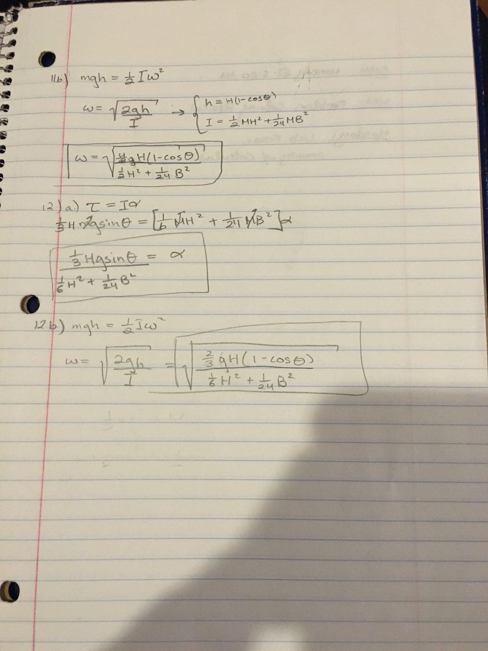We then changed the mass of the disk and measured the angular acceleration. (See Figure 16.1) Part 2 involved deriving an expression (See Figure 16.2) and using that to find the frictional torque and inertia of the disk. (See Figure 16.3) Our theoretical and experimental inertias remain similar, but are on two different measurements. Theoretical calculations rely on the equation 1/2 MR^2, while experimental calculations rely on alpha and other measurements

Data Tables/Analysis:

Figure 16.1 - Table of different angular accelerations based on different masses and radii. We notice that the mass changes in a linear pattern according to either hanging weight or radius of torque pulley

Figure 16.2  - equation used to find the inertias of the objects. This equation assumes that there is no friction acting on the system.

Figure 16.3 - acceleration graphs

Conclusion: Our inertias are close, but like always there’s some uncertainty. Being that they are two different methods of reaching a similar answer, there is going to be some uncertainty in theoretical calculations and uncertainty in experimental calculations. For theoretical calculations, there are rounding errrors, measurement errors, and we are assuming that the disks are solid rather than hollow. Whereas in our experimental data, we assume that the torque due to friction is the same in all directions and is independent of omega. We also assume that there is some uncertainty in our alpha as we did have to average it, therefore, changing the nonconstant alpha.

Lab 17: Finding the moment of inertia of a uniform triangle about its center of mass

Lab 17: Finding the moment of inertia of a uniform triangle about its center of mass

Authors: Lab conducted by Mohammed Karim (author), Bemaya, and Loius.

Objective: Compare theoretical and experimental values of moments of inertia.

Theory/Intro: Using the parallel axis theorem, we can calculate inertia of the triangle at a certain point. In this experiment, we will find the moment of inertia of the pulley system alone, then attach the triangle, and measure it again. By subtracting the two moments of inertia, we can calculate the triangle alone and compare the results.

Apparatus/Procedure:

               Like lab 16, we are using the same mass-pulley system. First, we attached a mass and measured the average angular acceleration using LoggerPro. The value for the “empty” system was 2.186 rad/s^2. Next, we found the value for the triangle with the longer side up, as 2.0205 rad/s^2. Lastly, the value for the triangle with the longer side down, was 1.8375 rad/s^2. Using angular acceleration, we could calculate the experimental values for inertia. We then calculated the inertia through the parallel axis theorem (See Figure 17.1) and compared the results.

Data Tables:

Figure 17.1 - Calculations

Figure 17. 2 - Angular Acceleration Empty

Figure 17.3 - Angular Acceleration Triangle Up

Empty: 0.000278 kgm^2 (experimental)

Triangle up: 0.000236 kgm^2 (experimental), 0.0002444 kgm^2 (theoretical)

Triangle down: 0.0005374 kgm^2 (experimental), 0.0005672 kgm^2 (theoretical)

Analysis: The data shows the calculations behind finding the inertias of certain objects. Using the parallel axis theorem, we were able to find the theoretical data. By subtracting the empty pulley with the triangle pulley, we were able to find the inertia of the respective shape.  

Conclusion: This experiment expected us to get close values between our experimental and theoretical values. Our results are close; however, we are off by a small value. This could be primarily due to the uncertainty of the forces applied. There could have been little friction in one run and more friction in another. Also, there are many uncertainties relating to our calculations such as rounding and measuring errors, and we may have neglected factors such as friction and varying acceleration. As acceleration was not constant, we simply averaged it, which could have led to more uncertainty depending on the discrepancy of our values. 

Lab 18: Lab Problem – Moment of inertia and frictional torque

Lab 18: Lab Problem – Moment of inertia and frictional torque

Authors: Mohammed Karim, Bemaya, and Louis.

Objective: Find the frictional torque done by the wheel and determine the time it would take for a car tied to the wheel to slide down the track.

Theory/Intro: We understand that inertia acts as a system and, as a result, can ratio the values to find the mass and inertias of each individual object.

Apparatus/Procedure:

              

Pic of apparatus

               In this lab, we are given a metal disk that spins on a shaft and are tasked with making measurements of each of the parts. We then calculated the volume of each individual “cylinder” and used proportions to find the mass of the disk and the supports. (See Figure 18.1) Then, we recorded the spinning and marked it using LoggerPro to find the deceleration. This value, the angular deceleration due to friction, was 0.5551 rad/s^2. We then calculated the torque due to friction (See Figure 18.2) Now that we had the frictional values, we could run the car down the 1 meter track. We set up a sum of force equation and concluded that the car would have an acceleration of 0.0333 meters/second^2. Finally, by using kinematics, our theoretical time for the time it would take the car to travel 1 meter was 7.76s. (See Figure 18.3) After running the experiment, our experimental value was a bit lower than our theoretical value, but by less than 4%.

Data Tables/Analysis:

Figure 18.1 - Calculation for the mass of the metal disk and the torque due to friction

Figure 18.2 - Value for frictional deceleration (off by a factor of 10; did not do meters)

Figure 18.3 - Calculations for the time it would take the cart to travel 1 meter

Conclusion: This lab, being a giant problem, is basically a two part question, in which first you must find the frictional torque behind the spinning of the wheel, then you must use it to calculate the acceleration of the car and, as a result, the time it takes the car to travel one meter. Overall, our theoretical value was very close to our experimental value, but could be off due to the uncertainty of our calculations, the uncertainty behind the ratios of mass to volume, the uncertainty behind the angle the track makes with the horizontal, and the fact that we neglected the friction due to the track and the car. However, if these values were considered, we would have seen a far more precise answer.

Experiment 8: Conservation of Angular Momentum

Experiment 8: Conservation of Angular Momentum

Authors: Lab conducted by Mohammed Karim (author), Richard, and Lynel.

Objective: Use conservation of momentum to find the angular acceleration of the disk.

Theory/Intro: During collision, we know that momentum is always conserved. Therefore, if we wanted to find the angular acceleration of a disk when being hit by a ball, we can find a solution if we have the velocity at which the ball hits the disk.

Apparatus/Procedure:

              

See pic of apparatus

               Our first step before calculating the angular acceleration, would be to calculate the velocity at which the ball hits the disk. We solved this by rolling the ball on the same ramp off the table and finding the distance it landed. (See Figure 19.1) After marking the distance from and height from the table and the carbon paper that the ball landed on, we could calculate the velocity through kinematics. The equation v=L/sqroot(2h/g) gave us a velocity of 1.3301 m/s. Next, after taking the measurements of the disk and finding the velocity, we could conduct the experiment. Using LoggerPro, we received a value of 5.5545 rad/s^2. (See Figure 19.2) We conducted multiple trial runs so we can see the affects of landing at different radii.

Data Tables:

Figure 19.1 - Drawing of setup with measurements

Figure 19.2 - Trial Run 1

Figure 19.3 -Trial Run 2

Figure 19.4 - Trial Run 3 ft. Prof Wolf

Analysis: We can see the relationship between angular momentum and the radius at where the ball lands. By doing many trials, we see that the further the ball goes, the faster the disk will spin. This is in line with what we know about torque. The further the force is applied on the radius, the more torque there is. We are able to determine values such as the gravitational potential energy of the ball. Starting from a height above due to the ramp, it definitely has potential energy. As it leaves, it has a velocity, therefore, it has a kinetic energy. Lastly, as it is rolling without slipping, it has rotational kinetic energy.

Conclusion: This experiment shows the conservation of angular momentum in a disk system. We understand that angular momentum is conserved, however, the analysis discusses energy, and the question to ask is, “Is energy conserved?” The answer to this question would be no. Especially in real life experimentation, energy is not conserved. For one, there is friction on the track that causes the ball to roll without slipping and occasionally slip. When the ball collides, energy is not necessarily conserved either as they ball collides into the platform and may have jolted or bounced and as a result, lost energy. Therefore, energy was not conserved. 

Lab 19: Conservation of Energy/Conservation of Angular Momentum

Lab 19: Conservation of Energy/Conservation of Angular Momentum

Authors: Lab conducted by Mohammed Karim, Richard, and Lynel.

Objective: Compare experimental and theoretical results to the height that the clay/meter stick system raise to.

Theory/Intro: Using energy and angular momentum, we can calculate the height that the meter stick rises to. Now, we test our mastery in two physics concepts and see how accurate our calculations can be.

Apparatus/Procedure:

               Pic of apparatus

               The lab is set up to contain a meter stick, pivoted at the 10-cm mark, dropped from a height of 0.4m. It then collides with some clay and raises to a certain height. This can be calculated by splitting the problem into three parts. The first part is using the energy theorem to calculate the angular speed at which the meter stick hits the clay. (See Figure 19.1) Next, we calculate the final angular speed after the collision through conservation of angular momentum. (See Figure 19.1) Once we have the angular speed, we then calculate height by using the energy theorem once again. (See Figure 19.2) After calculating a theoretical value for height (0.3m), we put our math to the test and used motion tracking to calculate the maximum height of the meter stick and were able to come up with an experimental value of 0.363.

Data Tables/Analysis:

Figure 19.1 - Contains conservation of energy part 1 and conservation of angular momentum. For cons of energy, we found an omega. We used that omega in our angular momentum equation.

Figure 19.2 - Once we have the omega final, we plug it in to one last conservation of energy equation. This equation is done to calculate the height of the clay-stick system.

Conclusion: Our data came out pretty accurate. However, it is surprising that our experimental data was greater than our theoretical data. Usually, when conducting our experiments, our experimental data is typically smaller due to neglecting friction or some factor. However, this time it seems to be greater. My hypothesis is that the error is a result of multiple factors. For one, there could have been a slight intial force given to the meter stick as opposed to it being released from rest. Another reason could be that our points were not plotted at the exact center of mass of the meter stick/clay system. Alternatively, our collision may have altered it. Although it was an actual collision, the stick was mainly from the adhesive tape. However, I wouldn’t be too confident in saying that would result in the stick going much higher. Lastly, there is the consistent rounding error, but that would account for a very minor error. 

Lab: Physical Pendulum

Lab: Physical Pendulum

Authors: Lab conducted by Mohammed Karim (author) and Richard.

Objective: Find the period of different physical pendulums with varying inertia.

Theory/Intro: We understand that varying inertia affect the angular acceleration. Now, with the new concepts of simple harmonic motion and oscillations, we will see how different inertia affect the oscillations involved in the period of a single oscillation.

Apparatus/Procedure:

              

Post pic of apparatus

               First, we were tasked with calculating the inertia for six different figure orientations as a prelab. (See Figure 20.1) When we had this value, we were able to continue with the procedure. Using the values of inertia, we found the period through a torque equation. We then compared this theoretical result with our experimental result. How we calculated our experimental period was by placing a photogate underneath the oscillating object, where it would track the oscillations by the tape that stuck out. The first object that we dealt with was a ring. This ring was treated as a point mass a distance r away from the radius. We solved the angular frequency and time by using the equation T= 2(pi)/omega where omega is sqroot(g/2r), and found a theoretical value of 1.06s. This was very close to our 1.07 value that we tested using the pendulum. Next, we had to calculate the expression for the period of each isosceles triangles oriented at the apex and midpoint of the base. (See Figure 20.2) As you can see, our theoretical values for time were 0.6503 and 0.5728 seconds, respectively. As for our experimental data, we received experimental values of 0.6574 and 0.5946 seconds.

Data Tables/Analysis:

Figure 20.1 - Inertia and Angular acceleration calculations for triangles (Circles not included as we did not use them for lab)

 
 

Figure 20.2- period calculations of the isosceles triangle

Experimental graph of Period of Isosceles around apex:

Experimental of Isosceles around Base

Conclusion: This lab was straightforward. We calculated the inertia, used that to find angular acceleration through a torque equation, found the value of angular frequency, and calculated the period. After finding a value, we compared our theoretical and experimental values and were extremely accurate. Practically to the nearest percent, if not closer. Our values would have been exact had our degree of oscillation been slightly less, due to us discounting sin (theta). Another uncertainty that could have affected our data would be the axis of tilt, certain shapes were not perfectly even and straight and as a result, oscillated at some angle. However, for the most part, it was really accurate and hard to complain about with such precision. Specifically, for the first part, we assumed that the ring is a point mass, a distance r away from the center, however, it is more of an inner outer radius. In order to get a much closer result, we would use (1/2M(Ro^2+Ri^2))

Lab: Ballistic Pendulum

1.     Lab: Ballistic Pendulum

a.      Lab conducted by Mohammed Karim (author)

2.     Objective –  There were two objectives to this lab. The first being to calculate the initial velocity that the bullet fires into the box, and the second being to prove that the velocity is correct by using the velocity to calculate the distance the ball will travel.

3.     Theory/Introduction – Knowing various concepts like projectile motion, energy, and momentum, can help us accomplish even the most complex of problem. In this lab, we are tasked with finding the initial velocity that the bullet fires into the box, given the length of the “string” and the angle the box travels.  

4.     Apparatus/Procedure –

     The apparatus is pretty much a ready made pendulum. We fired it multiple times, found the average theta, length of the “string”, mass of the bullet, and mass of the box. We then solved for velocity initial of the bullet, which turned out to be 4.837 m/s (See Figure 14.1 for calculations). In order to put this answer to the test, we calculated the distance it would travel before it hits the floor, using the velocity we calculated. We first found time using h=1/2gt^2, and then plugged it into x=vt, giving us 2.1945m. After firing the shot, we got around 2.35-2.43m (See Figure 14.2 for calculations)

5.     Data Tables

Figure 14.1 – Calculation of the initial velocity of the bullet.

Figure 14.2 – Calculations of the distance of the bullet using projectile motion.

6.     Conclusion – Overall, our results were very accurate as our calculations were around 5 percent of our experiment. This is a victory in my book. Had there not been many uncertainties, I would have been 100% correct. These uncertainties include, rounding up values during the multiple calculations, air resistance, uncertainty of force used when firing with the cannon, and uncertainty in measurement of the height and distance the cannon was from the point of impact. Had these little values been exact, I think my answer would have been much closer, if not the same.

Lab 13: Magnetic Conservation of Energy

1.     Lab 13: Magnetic Conservation of Energy

a.      Lab conducted by Mohammed Karim (author), and Lynel.

2.     Objective –  Derive an equation that can be used for magnetic potential energy. First, find an equation, using a power fit, for force and integrate for magnetic potential energy.

3.     Theory/Introduction – Prior to this lab, we have equations that are modeled after change in height and speed and even springs. However, we don’t have anything that relates position and magnetic forces. This lab will aim to find an equation that can be used.

4.     Apparatus/Procedure

           The apparatus is a track in which the carts can glide through. Air is blown into the track so that it can model a frictionless track. What we did was attach a magnet to the end of the track and the cart. We then move the cart toward the magnet and record the distance the magnet keeps the block from it. We did this over the course of many different angles until we had enough data to plot our data. We set this data up as a power fit and integrated it to find the work.

5.     Data Tables

Figure 13.1 – Shows power fit. The values are all found in the box. This is the Force of the magnet. If it is integrated, we get the equation for magnetic potential energy.

Figure 13.2 - Shows the values of theta and r, being the distance from the magnet.

Figure 13.3 – Shows the total energy and conservation of energy in the system.

6.     Conclusion – We accurately modeled an equation for magnetic potential energy. As this was part of conservation of energy, we see that this also fits into the whole conserved energy graph shown in figure 13.3 accurately. Of course the total energy wasn’t fully conserved as there was some friction in the air track and certain uncertainties in the value could have altered it, but for the most part, the graph fits in.

Lab 12: Conservation of Energy – Mass Spring System

1.     Lab 12: Conservation of Energy – Mass Spring System

a.      Lab conducted by Mohammed Karim (author), Lynel, Andrew, and Richard.

2.     Objective –  Understand conservation of energy and the different forms of energy the system takes depending on position, height, speed, and force.

3.     Theory/Introduction – As if Physics wasn’t hard enough, we’ve decided to throw Calculus into it. One may ask themselves why? Well, because life is less than ideal. Not every mass is uniform and the gravitational potential energy is not always just mgh. As shown in figures 12.1 and 12.2, the calculations and derivations are done in detail to give us the equations we will be using. We need to keep in mind that in a hanging spring system, there are five forms of energy acting on it. There is gravitational potential energy of the hanging mass, kinetic energy of the hanging mass, elastic potential energy of the spring, gravitational potential energy of the spring, and kinetic energy of the spring. These values need to be kept in mind when we are conducting the following experiments.

4.     Apparatus/Procedure – Explain Apparatus and Procedure

           The apparatus above shows a spring hanging vertically with a mass tied onto it. There is a force sensor on top of the system, and on there is a motion sensor on the floor. With these, we will be detecting force and distance with respect to time. We then stretch the spring and allow it to oscillate, while running the various sensor to give us necessary data to plot a few graphs. After conducting the experiment, we plotted position, velocity, kinetic energy, gravitational potential energy, and elastic potential energy. (See Figures 12.3-12.6)

5.     Data Tables

Figure 12.1 - pt. 1/2 - Calculus required to find out energy equations with realistic conditions.

Figure 12.2 - pt. 2/2 - Calculus required to find out energy equations with realistic conditions.

Figure 12.3 Elastic potential energy vs. position and velocity graph. It shows the relation between position near equilibrium and potential energy.

Figure 12.4 Gravitational potential energy over position and velocity. GPE, being related directly with height, varies with position.

Figure 12.5 Kinetic Energy over position and velocity graphs. Shows the balance and how when velocity is zero, kinetic energy is and when velocity is at its peak, kinetic energy is as well.

Figure 12.6 - position over time and velocity over time graphs. The simple building blocks used to find the energy graphs.

6.     Conclusion – Conservation of energy is a very cool concept in the sense that it is very easy to follow. Energy is always in the system and is not lost (unless its due to heat or some other form). Therefore, if one energy is not present, the other form will have a lot more energy. This is shown in the graphs above. In the system, when it reaches the top or bottom, velocity is zero. Therefore, energy is zero, however, gravitational and magnetic potential are very high. When the object is at an equilibrium point, the velocity is at its highest, meaning kinetic energy is very high. 

Lab 11 - Work-Kinetic Energy Theorem Lab

1.     Lab 11: Work-Kinetic Energy Theorem Activity

a.      Lab conducted by Mohammed Karim (author), Lynel, Andrew, and Richard.

2.     Objective –  This lab contained two parts. The first part dealt with finding the work done by a nonconstant spring force. Basically, we were to find the work done by stretching a spring with a cart. The second part dealt with the work kinetic energy principle. Our goal was to relate force and position and kinetic energy and position.

3.     Theory/Introduction – We know the work is force * distance or the area under the curve of a force * distance graph. If we were to calculate the force over position of a cart opposing a spring and integrate it, we could find the work done. Next, we can take another similar scenario and relate position and kinetic energy as the work done by the spring force can be related to kinetic energy as explained by the work kinetic energy theorem.

4.     Apparatus/Procedure – Explain Apparatus and Procedure

The apparatus above features a cart on a track attached to a spring. We used a force probe to measure the force applied. We measured the position and moved the cart 0.6 meters and plotted our values on a force over position. After plotting it, we found the slope of the tangent line and measured the area under the curve. (See figures 11.1 and 11.2). The slope of the tangent line would be our spring constant. (8.828 N/m). The area under the curve of the graph would be the work done.

     As for the second experiment, we placed a 0.7+/- 0.01kg cart on a track with a stretched spring attached to it. We then measured the compression of the spring as it goes back to a state of equilibrium. We took the values of Force, position, and kinetic energy and graphed them to see the relationship (See Figure 11.3)

5.     Data Tables

Figure 11.1 – Picture of the slope of the tangent line. The m value, or the slope, is the spring constant used in equations involving a spring and work/force.

Figure 11.2 – Picture of the area under the curve. The area represents the work done.

Figure 11.3 – Graph of Force over position and Kinetic Energy over position

Any data tables/pictures referred to during experiment.

6.     Conclusion – The graphs from this activity/lab relate many important concepts. From a “graph” standpoint, it helped me understand the relation and derivation for certain values and equations. Aside from work is the integral of force with respect to time, I found out some new information, such as the value k, the spring constant, is found through the slope of the tangent line of the force vs. position graph. I now see the relationship between force and kinetic energy, as shown by the graphs. This relates the work kinetic energy theorem. As force vs position increases, kinetic energy decreases.