Lab: Ballistic Pendulum

1.     Lab: Ballistic Pendulum

a.      Lab conducted by Mohammed Karim (author)

2.     Objective –  There were two objectives to this lab. The first being to calculate the initial velocity that the bullet fires into the box, and the second being to prove that the velocity is correct by using the velocity to calculate the distance the ball will travel.

3.     Theory/Introduction – Knowing various concepts like projectile motion, energy, and momentum, can help us accomplish even the most complex of problem. In this lab, we are tasked with finding the initial velocity that the bullet fires into the box, given the length of the “string” and the angle the box travels.  

4.     Apparatus/Procedure –

     The apparatus is pretty much a ready made pendulum. We fired it multiple times, found the average theta, length of the “string”, mass of the bullet, and mass of the box. We then solved for velocity initial of the bullet, which turned out to be 4.837 m/s (See Figure 14.1 for calculations). In order to put this answer to the test, we calculated the distance it would travel before it hits the floor, using the velocity we calculated. We first found time using h=1/2gt^2, and then plugged it into x=vt, giving us 2.1945m. After firing the shot, we got around 2.35-2.43m (See Figure 14.2 for calculations)

5.     Data Tables

Figure 14.1 – Calculation of the initial velocity of the bullet.

Figure 14.2 – Calculations of the distance of the bullet using projectile motion.

6.     Conclusion – Overall, our results were very accurate as our calculations were around 5 percent of our experiment. This is a victory in my book. Had there not been many uncertainties, I would have been 100% correct. These uncertainties include, rounding up values during the multiple calculations, air resistance, uncertainty of force used when firing with the cannon, and uncertainty in measurement of the height and distance the cannon was from the point of impact. Had these little values been exact, I think my answer would have been much closer, if not the same.

Lab 13: Magnetic Conservation of Energy

1.     Lab 13: Magnetic Conservation of Energy

a.      Lab conducted by Mohammed Karim (author), and Lynel.

2.     Objective –  Derive an equation that can be used for magnetic potential energy. First, find an equation, using a power fit, for force and integrate for magnetic potential energy.

3.     Theory/Introduction – Prior to this lab, we have equations that are modeled after change in height and speed and even springs. However, we don’t have anything that relates position and magnetic forces. This lab will aim to find an equation that can be used.

4.     Apparatus/Procedure

           The apparatus is a track in which the carts can glide through. Air is blown into the track so that it can model a frictionless track. What we did was attach a magnet to the end of the track and the cart. We then move the cart toward the magnet and record the distance the magnet keeps the block from it. We did this over the course of many different angles until we had enough data to plot our data. We set this data up as a power fit and integrated it to find the work.

5.     Data Tables

Figure 13.1 – Shows power fit. The values are all found in the box. This is the Force of the magnet. If it is integrated, we get the equation for magnetic potential energy.

Figure 13.2 - Shows the values of theta and r, being the distance from the magnet.

Figure 13.3 – Shows the total energy and conservation of energy in the system.

6.     Conclusion – We accurately modeled an equation for magnetic potential energy. As this was part of conservation of energy, we see that this also fits into the whole conserved energy graph shown in figure 13.3 accurately. Of course the total energy wasn’t fully conserved as there was some friction in the air track and certain uncertainties in the value could have altered it, but for the most part, the graph fits in.

Lab 12: Conservation of Energy – Mass Spring System

1.     Lab 12: Conservation of Energy – Mass Spring System

a.      Lab conducted by Mohammed Karim (author), Lynel, Andrew, and Richard.

2.     Objective –  Understand conservation of energy and the different forms of energy the system takes depending on position, height, speed, and force.

3.     Theory/Introduction – As if Physics wasn’t hard enough, we’ve decided to throw Calculus into it. One may ask themselves why? Well, because life is less than ideal. Not every mass is uniform and the gravitational potential energy is not always just mgh. As shown in figures 12.1 and 12.2, the calculations and derivations are done in detail to give us the equations we will be using. We need to keep in mind that in a hanging spring system, there are five forms of energy acting on it. There is gravitational potential energy of the hanging mass, kinetic energy of the hanging mass, elastic potential energy of the spring, gravitational potential energy of the spring, and kinetic energy of the spring. These values need to be kept in mind when we are conducting the following experiments.

4.     Apparatus/Procedure – Explain Apparatus and Procedure

           The apparatus above shows a spring hanging vertically with a mass tied onto it. There is a force sensor on top of the system, and on there is a motion sensor on the floor. With these, we will be detecting force and distance with respect to time. We then stretch the spring and allow it to oscillate, while running the various sensor to give us necessary data to plot a few graphs. After conducting the experiment, we plotted position, velocity, kinetic energy, gravitational potential energy, and elastic potential energy. (See Figures 12.3-12.6)

5.     Data Tables

Figure 12.1 - pt. 1/2 - Calculus required to find out energy equations with realistic conditions.

Figure 12.2 - pt. 2/2 - Calculus required to find out energy equations with realistic conditions.

Figure 12.3 Elastic potential energy vs. position and velocity graph. It shows the relation between position near equilibrium and potential energy.

Figure 12.4 Gravitational potential energy over position and velocity. GPE, being related directly with height, varies with position.

Figure 12.5 Kinetic Energy over position and velocity graphs. Shows the balance and how when velocity is zero, kinetic energy is and when velocity is at its peak, kinetic energy is as well.

Figure 12.6 - position over time and velocity over time graphs. The simple building blocks used to find the energy graphs.

6.     Conclusion – Conservation of energy is a very cool concept in the sense that it is very easy to follow. Energy is always in the system and is not lost (unless its due to heat or some other form). Therefore, if one energy is not present, the other form will have a lot more energy. This is shown in the graphs above. In the system, when it reaches the top or bottom, velocity is zero. Therefore, energy is zero, however, gravitational and magnetic potential are very high. When the object is at an equilibrium point, the velocity is at its highest, meaning kinetic energy is very high. 

Lab 11 - Work-Kinetic Energy Theorem Lab

1.     Lab 11: Work-Kinetic Energy Theorem Activity

a.      Lab conducted by Mohammed Karim (author), Lynel, Andrew, and Richard.

2.     Objective –  This lab contained two parts. The first part dealt with finding the work done by a nonconstant spring force. Basically, we were to find the work done by stretching a spring with a cart. The second part dealt with the work kinetic energy principle. Our goal was to relate force and position and kinetic energy and position.

3.     Theory/Introduction – We know the work is force * distance or the area under the curve of a force * distance graph. If we were to calculate the force over position of a cart opposing a spring and integrate it, we could find the work done. Next, we can take another similar scenario and relate position and kinetic energy as the work done by the spring force can be related to kinetic energy as explained by the work kinetic energy theorem.

4.     Apparatus/Procedure – Explain Apparatus and Procedure

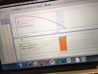
The apparatus above features a cart on a track attached to a spring. We used a force probe to measure the force applied. We measured the position and moved the cart 0.6 meters and plotted our values on a force over position. After plotting it, we found the slope of the tangent line and measured the area under the curve. (See figures 11.1 and 11.2). The slope of the tangent line would be our spring constant. (8.828 N/m). The area under the curve of the graph would be the work done.

     As for the second experiment, we placed a 0.7+/- 0.01kg cart on a track with a stretched spring attached to it. We then measured the compression of the spring as it goes back to a state of equilibrium. We took the values of Force, position, and kinetic energy and graphed them to see the relationship (See Figure 11.3)

5.     Data Tables

Figure 11.1 – Picture of the slope of the tangent line. The m value, or the slope, is the spring constant used in equations involving a spring and work/force.

Figure 11.2 – Picture of the area under the curve. The area represents the work done.

Figure 11.3 – Graph of Force over position and Kinetic Energy over position

Any data tables/pictures referred to during experiment.

6.     Conclusion – The graphs from this activity/lab relate many important concepts. From a “graph” standpoint, it helped me understand the relation and derivation for certain values and equations. Aside from work is the integral of force with respect to time, I found out some new information, such as the value k, the spring constant, is found through the slope of the tangent line of the force vs. position graph. I now see the relationship between force and kinetic energy, as shown by the graphs. This relates the work kinetic energy theorem. As force vs position increases, kinetic energy decreases. 

Lab 9: Centripetal Force with a Motor

1.     Lab 9: Centripetal force with a motor

a.      Lab conducted by Mohammed Karim (author), Lynel, Richard, and Andrew.

2.     Objective –  Understand the relationship between theta (degree shown in Figure 9.1/9.2) and create a working linear equation that can be used to find the value.

3.     Theory/Introduction – We understand that the manipulation of force can cause an object to swing with a certain angle with respect to the ground. When an object connected to a string is dormant, it is perpendicular to the ground. However, as it spins faster and faster, the object begins to tilt toward the horizontal. Using the apparatus shown below, we are tasked with finding a fit.

4.     Apparatus/Procedure –

Apparatus.jpg

 

The apparatus shown above was the only apparatus used throughout the experiment. Basically, a mass hung from the string. The pole, that the string was connected to, began to spin with increasing velocities. The increasing velocities created a greater centripetal force, thereby increasing the tension and the angle it makes with the floor. We collected different values and used some trigonometry to find the angle the object made. We measured the distance the object was from the apparatus, and the height it was at. We then found the adjacent component and found the angle the string made with arccos. (Keep in mind that the length of the string was constant.) An example can be seen in figure 9.2.

After finding the values for multiple test runs, we plugged in the values on excel and loggerpro. (see figures 9.3 and 9.4) We then compared this to the conceptual data we had calculated and graphed it. (see figure 9.5)

5.     Data Tables

Figure 9.2

Figure 9.3

Figure 9.4

Figure 9.5.

6.     Conclusion – Overall, the conceptual data and experimental data were very close. The graph had a slow of 0.9371, showing that they were in line. Had the slope been a perfect one, the two results would have been the same. Of course, a much closer answer could have been reached, but like always, there were many factors that could have played a role in giving us a less than accurate result. One being the voltage that the object spins at as opposed to the velocity the object is at. This would be hard to fix as that would be more complex physics information. Another uncertainty would be wind resistance as the object is spinning fast and the friction from the wind could affect the objects ability to reach top speed, thus lowering its overall height. There is also propagated uncertainty in our measurements with height and where exactly the object should touch the ruler. These small percentages, while they may seem small can add and give us a much more precise answer. Even if there was a five percent uncertainty, that could put us at a 0.99 correlation, which would essentially show that the experimental data and conceptual data are the same. 

Lab 8 Centripetal Acceleration vs. Angular Frequency

1.      Lab 8: Centripetal Acceleration vs. Angular Frequency (not in lab book)

a.      Lab conducted by Mohammed Karim (author), Lynel, Andrew, Richard

2.      Objective –  Better understand the variables behind centripetal acceleration and how changing a variable affects the overall result.

3.      Theory/Introduction – Centripetal acceleration is comprised of mass*radius*omega^2. In this lab, we change the values in excel and solve the centripetal acceleration.

4.      Apparatus/Procedure –

There was a single apparatus used. It consisted of a disk being spun by many tires. We attached a motion sensor at different points to affect the radius. We changed the masses to change mass (of course) and we changed the speed to affect omega. After changing the values, we wrote down the values and graphed them in excel.

5.      Data Tables

Shows the changing mass and how it affects force.

Shows the changing radii and changing velocities to affect omega.

6.      Conclusion – Overall, our results showed that changing mass and radius affects centripetal force linearly. If we changed omega, it changed the value based on a quadratic function (because it is squared). For example, if we were to double omega, it would multiply centripetal force by 4.

Lab 6 Propagated Uncertainty

1.      Lab 6: Propagated Uncertainty in measurements

a.      Lab conducted by Mohammed Karim (author), Curtis, and Lynel

2.      Objective –  Understand the role propagated uncertainty plays in our measurements and understand how to take into account this error and get more accurate results.

3.      Theory/Introduction – Prior to learning about propagated uncertainty, we didn’t have a way for us to fix any minor errors in our measurements. For example, if we measured a block that did not completely meet the centimeter mark, we would typically round it. This, while it may be a minor, could vastly skew the results, as much of the experiment relies on that measurement being accurate. If our measurement is slightly inaccurate, then we could be missing monumental concepts, such as energy not being conserved, momentum being conserved, etc.

4.      Apparatus/Procedure – There was no apparatus involved in this experiment aside from two cylinders in which we measured the height, mass, and diameter. (See Figure 6.1) Using these measurements, we found density. However, to consider the propagated uncertainty, we used an equation to get the uncertainty. (See Figures 6.2, 6.3) The final step would just be to assemble our results, as shown in Figure 6.4.

5.      Data Tables

Any data tables/pictures referred to during experiment.

6.      Conclusion – This lab was fairly short as there wasn’t much to do besides calculate propagated uncertainty. Personally, it does feel much better to be able to get a much more accurate result and become more advanced when conducting future experiments.